Clean/Filter Data
2024-02-01
Source:vignettes/MoveR-Clean-FilterData.Rmd
MoveR-Clean-FilterData.RmdNow that we are familiar with importing raw data from tracking software, we are focusing on how to clean/filter them.
For this example we are selecting the second sample of data available in the MoveR_SampleData github repository.
Briefly, this dataset comes from the video recording (image resolution: 1920x1080) of 24 parasitic micro-wasp individuals (genus Trichogramma) placed in a thermostated circular arena (2.5cm diameter, see Ion Scotta et al., 2021) for 110 minutes at 25 fps (see fig. 1 left panel).
Over the exposure duration individuals has been exposed to a steady increases in temperature from 18℃ to 45℃ followed by a steady decreases from 45℃ to 18℃ (temperature changing rate: 0.5℃ per minutes). Individuals were then tracked using TRex (Walter and Couzin, 2021).
To reduce space allocation and computing time we reduced the dataset by removing the movements recorded below 35℃ (see fig. 1 right panel).


Figure 1: Frames extracted from a video recording of 24 parasitic micro-wasps (genus Trichogramma) placed in a thermostated circular arena (left). Temperature ramp over which the movements of parasitic micro-wasp were recorded. The shaded area corresponds to the part of the data removed from the original dataset (i.e., moments where temperature was below 35℃) while the white area correspond to the remaining data used in the following exemple (right).
Import sample data from github
Let’s download the data, import them as a tracklets object and specify some additional information that will be useful for this tutorial (i.e., frame rate, scale, image resolution) using setInfo() (see the Import Data vignette for detailed procedure).
Note that we have included some extra data that are related to this dataset within the “raw tracking data” when we have reduced the dataset:
These extra information will be useful to conduct further analyses in this tutorial and some others.
As the number of elements returned by TRex is relatively high and is not helpful here, we also are removing some of them by keeping only the necessary elements (maj.ax, x.pos, y.pos, identity, frame, runTimelinef and Measured_Temp_Deg_C). To ease this process we can first convert the tracklet object to a list of variable (varList object) using convert2List(), select only the desired variables and convert the varList back to tracklets using convert2Tracklets().
Note that additional the information added to the tracklets object are conserved over the conversion process using convert2List() and convert2Tracklets().
# dl the second dataset from the sample data repository
Path2Data <- MoveR::DLsampleData(dataSet = 2, tracker = "TRex")

# Import the sample data
TRexDat <- MoveR::readTrex(Path2Data[[1]],
                           rawDat = T)

# set additional information within the tracklets object (frameR is already retrieved from TREx data). In this video 1 cm represent 413.4 pixels (measured using the arena diameter -2.5cm- and ImageJ software https://imagej.net/ij/index.html).
TRexDat <- MoveR::setInfo(TRexDat, scale = 1/413.4, imgRes = c(1920, 1080))

# keep only the elements that will be useful for this tutorial (the timeline in frames and the temperature)
## convert the tracklets object into a variable list to ease the selection of desired variables
trackDatList <- MoveR::convert2List(TRexDat)
trackDatList <-
  trackDatList[c(
    "maj.ax",
    "x.pos",
    "y.pos",
    "identity",
    "frame",
    "runTimelinef",
    "Measured_Temp_Deg_C"
    )]

## convert it back to a tracklets object (conserving the additional information previously added)
trackDat <- MoveR::convert2Tracklets(trackDatList, by = "identity")
Now we have imported the data, we can clean them to remove for instance:
infinite values corresponding to the moments where the particles were undetected
probable spurious elements detected by the tracking software using several filters based on the particles size, speed, location within the arena).
For this purpose, 3 main functions, filterFunc(), mergeFilters() and filterTracklets() allow to specify custom filters, merge several filters and use them to clean the data, respectively.
Remove infinite values
Infinite values are added by TRex when the particles are temporarily undetected, the following code help to remove infinite value and split the trajectories carrying them accordingly.
In other words, when a particle is temporarily undetected we assume that the identity of the tracklet is spurious (conservative approach), thus the function create a new tracklet with a new identity (trackletId). Nevertheless, the original identity of the particles is still conserved in the “identity” vector.
Because infinite values can be detected in both x and y coordinates (i.e., x.pos and y.pos) we are using filterFunc() to create the filters on each variable and then mergeFilter() to combine the two filters.
# specify the filter to detected infinite values on "x.pos"
filter.InfX <-
  MoveR::filterFunc(
    trackDat,
    toFilter = "x.pos",
    customFunc = function(x)
      is.infinite(x)
  )

# it is also possible to group two or more filter by using the mergeFilter function
# for instance by merging the result of several condition tests, here the detection of infinite value in "x.pos" and "y.pos".

## first specify the second filter
filter.InfY <-
  MoveR::filterFunc(
    trackDat,
    toFilter = "y.pos",
    customFunc = function(x)
      is.infinite(x)
  )

## then merge the previously specifed filter
filter.Inf <-
  MoveR::mergeFilters(filters = list(filter.InfX, filter.InfY),
                     cond = TRUE)
Now, that the filter is properly specified the dataset can be filtered to remove infinite values detected on both x and y coordinates using filterTracklets().
Note that in case a particle is lost and detected again during a very short time period, the function may return small tracklets which may be considered useless. These small tracklets can be removed by specifying the minimum duration above which tracklet should be kept using the minDur argument.
For this example, we are keeping only the tracklets lasting more than one second by setting minDur to 25 frames which correspond to 1 second, or to the frame rate of the video (hence we can use the frameR attribute that is contained in the tracklets object).
# filter infinite values according to the previously specified filters
# here we are also removing the tracklets that are shorter than 25 frames (1 second) using the minDur argument.
trackDat.Infilt <-
  MoveR::filterTracklets(trackDat,
                     filter = filter.Inf,
                     splitCond = TRUE,
                     minDur = MoveR::getInfo(trackDat, "frameR"))

# display the summary of the filtering process
str(trackDat.Infilt[[1]])
## List of 8
## $ Tracknb_before_filter : int 88
## $ Tracknb_after_filter : int 165583
## $ Tracknb_after_minDur : int 6724
## $ TotTrackDuration_before_filter: int 4716398
## $ TotTrackDuration_after_filter : int 1664533
## $ TotTrackDuration_after_minDur : int 1177729
## $ %Data_kept_after_filter : num 35.3
## $ %Data_kept_after_minDur : num 25The function output correspond to a list containing 2 sublists:
the first one being a summary of the filtering process
the second containing the list of filtered tracklets which can be used for further computation
See the help page of the function for more details (filterTracklets())
According to the summary of the filtering process the number of tracklet drastically increases after the filtering (Tracknb_before_filter = 88 -> Tracknb_after_filter = 165583 tracklets). However a large amount appears to be very short which may be due to punctual detection of an individual over the timeline.
This observation is confirmed because specifying the minDur argument removed an important part of these tracklets (Tracknb_after_filter = 165583 -> Tracknb_after_minDur = 6989 tracklets).
Hence, there is a lot of moments where the micro-wasps were undetected within the dataset. As results, the filtering removed 64.7% (100-35.3) of the data corresponding to infinite values and then removed another 10.2% (35.3-25.1) because the resulting tracklets were shorter than 1 second (25 frames).
Now that we have removed the infinite values from the dataset, we can identify spurious detection by filtering on particles size.
Filter based on particles size
To remove the spurious detection of particles generated over the video-tracking procedure, one cleaning step can consist on removing all the moment when a particles’ size is lower or higher than a given threshold (e.g., the known size of the animals).
We first retrieve the scaling of the video using the diameter of the circular arena measuring 2.5cm and it’s length in pixels.
Then, we know that Trichogramma’s body length is generally higher than 0.15mm and lower than 1mm (personal observation) we can hence use these limits to filter the particles for which the length is not included within this interval (fig. 2A&B).
# the upper and lower limits to filter on particles length, according to the scale (expressed in cm)
LengthLim <- c(0.015, 0.1)

# convert the previously filtered data into a list to ease particle's size conversion (from pixels to cm)
trackDat.InfiltList <-  MoveR::convert2List(trackDat.Infilt[[2]])

# Use analyseTracklets function to scale the length of the particles (maj.ax) in cm by iterating over the tracklets
trackDat2 <- MoveR::analyseTracklets(trackDat.Infilt[[2]],
                                     customFunc =
                                       list(indLengthcm = function(x) x[["maj.ax"]] * MoveR::getInfo(trackDat.Infilt[[2]], "scale")))

# plot the distribution of particles' length (log10) and the size limits
par(mfrow=c(1,2))
hist(log10(MoveR::convert2List(trackDat2)[["indLengthcm"]]),
     breaks = 50,
     main = paste0("Particles' length (log10) and \ntreshold (cm)= ", LengthLim[1], "; ", LengthLim[2]),
     xlab = "Particles' length (log10)",
     cex.main = 0.8)
abline(v = log10(LengthLim), col = "firebrick")
mtext(substitute(paste(bold("A"))), side = 3, line = 0, adj = 0, padj = -0.5)

# create the filter
filter.length <-
  MoveR::filterFunc(
    trackDat2,
    toFilter = "indLengthcm",
    customFunc = function(x)
      x < LengthLim[1] | x > LengthLim[2]
  )

# apply the filter on the data using the frame rate as minimum duration of the tracklets
trackDat.lenfilt <-
  MoveR::filterTracklets(trackDat2,
                     filter.length,
                     splitCond = TRUE,
                     minDur = MoveR::getInfo(trackDat2, "frameR"))

# plot the distribution of particles' length (log10) after the filtering
hist(log10(MoveR::convert2List(trackDat.lenfilt[[2]])$maj.ax),
     breaks = 50,
     main = "Particles' length (log10) \nafter filtering",
     xlab = "Particles' length (log10)",
     cex.main = 0.8)
mtext(substitute(paste(bold("B"))), side = 3, line = 0, adj = 0, padj = -0.5)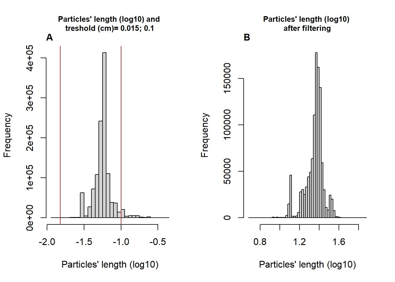
Figure 2: Histogram of the Log-transformed length of the particles and specified limits (vertical lines corresponding to 0.015 and 0.1 cm) of the distribution before (A) and after the filtering process (B) removing the moments where the particles’ length is below or above the specified limits.
# display the information about the filtering process (see ??filterTracklets())
str(trackDat.lenfilt[[1]])
## List of 8
## $ Tracknb_before_filter : int 6724
## $ Tracknb_after_filter : int 13997
## $ Tracknb_after_minDur : num 5520
## $ TotTrackDuration_before_filter: int 1177729
## $ TotTrackDuration_after_filter : int 1133835
## $ TotTrackDuration_after_minDur : int 1104334
## $ %Data_kept_after_filter : num 96.3
## $ %Data_kept_after_minDur : num 93.8According to the summary of the filtering step based on particles’ size, the amount of data removed by the filtering is reasonable with 3.7% of data considered above or below the particles’ length threshold.
However, the filter splited some tracklets in small part resulting in an additional 2.5% of data removed because resulting tracklets were shorter than 1 second (25 frames).
While the size of the particles is a good way to remove potential spurious detection, another efficient way to filter the data is based on the particles’ speed.
Filter based on particles speed
Indeed, the particles’ speed can be a good indicator of spurious detection or particle identification. More particularly, When the speed of a particle is too high (and have hence no biological meaning) it can be due to change in particle identity or more generally tracking artifact.
However, While the data can be filtered based data that already exist into the raw output of the tracking software, here the speed of the particles is not included, and in any case it should be recomputed since we have modified the tracklets over the previous filtering processes.
For the sacks of this example we will use the 999th percentile as a treshold above which particles’ speed are considered artifactual.
# retrieve the previously filtered data and used them to compute particles' speed
trackDat3 <- trackDat.lenfilt[[2]]

# Use analyseTracklets function to compute the speed of the particles by iterating over the tracklets
# here we use the "speed()" modulus to compute the speed over each tracklet
trackDat3 <-
  MoveR::analyseTracklets(trackDat3,
                      customFunc = list(
                        speed = function(x)
                          MoveR::speed(
                            x,
                            timeCol = "runTimelinef",
                            scale = 1
                          )
                      ))

# retrieve the speed of all particles in a vector
particleSpeed <- MoveR::convert2List(trackDat3)[["speed"]]

# compute the 999th percentile of particles' speed (log10 transformed data)
quant999th <- quantile(log10(particleSpeed), c(0.999), na.rm = T)

# plot the particles' speed (log10) distribution and the 999th percentile before filtering
par(mfrow=c(1,2))
hist(log10(particleSpeed), breaks = 100, main = "particles' speed (log10) and 999th quantile \nbefore filtering",
     cex.main= 0.9,
     xlab = "Particles' speed (log10)")
abline(v = quant999th, col = "#660000")
mtext(substitute(paste(bold("A"))), side = 3, line = 0, adj = 0, padj = -0.5)

# the result seem satisfactory since with this threshold we will remove only the few moments where particles speed overpass 22.5 pixels per frame while we conserve the bimodal distribution of the particles' speed.
# hence, create the filter based on the computed 999th quantile
filter.speed <-
  MoveR::filterFunc(
    trackDat3,
    toFilter = "speed",
    customFunc = function(x)
      x < 0 | x > 10 ^ quant999th
  )

# apply the filter on the data using the frame rate as minimum duration of the tracklets
trackDat.speedfilt <-
  MoveR::filterTracklets(trackDat3,
                     filter.speed,
                     splitCond = TRUE,
                     minDur = MoveR::getInfo(trackDat3, "frameR"))

# plot particles' speed (log10) distribution after the filtering
hist(log10(MoveR::convert2List(trackDat.speedfilt[[2]])[["speed"]]),
     breaks = 100,
     main = "Particles' speed (log10) \nafter filtering",
     cex.main= 0.9,
     xlab = "Particles' speed (log10)")
mtext(substitute(paste(bold("B"))), side = 3, line = 0, adj = 0, padj = -0.5)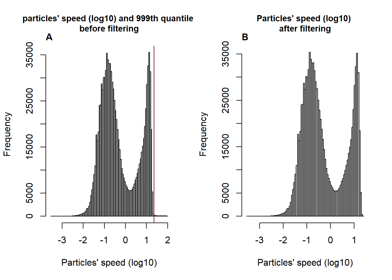
Figure 3: Histogram of the Log-transformed speed of the particles and 999th quantile (vertical line) of the distribution before (A) and after the filtering process (B) removing the moments where the particles’ speed is above the 999th quantile.
# display the information about the filtering process (see ??filterTracklets())
str(trackDat.speedfilt[[1]])
## List of 8
## $ Tracknb_before_filter : int 5520
## $ Tracknb_after_filter : int 6508
## $ Tracknb_after_minDur : num 5803
## $ TotTrackDuration_before_filter: int 1104334
## $ TotTrackDuration_after_filter : int 1103235
## $ TotTrackDuration_after_minDur : int 1094875
## $ %Data_kept_after_filter : num 99.9
## $ %Data_kept_after_minDur : num 99.1According to the summary of the filtering step based on particles’ speed, the amount of data removed by the filtering is reasonable with 0.1% of data considered above the speed threshold, which is consistent with our approach since we wanted to remove only extremes values (999Th quantile, fig. 3A&B).
Also, the filter splited only few tracklets in small part resulting in an additional 0.8% of data removed because resulting tracklets were shorter than 1 second (25 frames).
Finally, it seems interesting to remove the particles that are detected outside of the arena since it should be due to tracking artifact, or more generally to unintended particles’ detection and movements.
Filter based on particles detection outside the arena
Indeed, sometimes particles can be detected outside the arena, either because an individual as escaped from the arena or because the background has changed over the video recording (tracking artifact).
To solve this issue, it is possible to remove the parts of a tracklet that have been detected outside the arena.
To tackle this aim, one may either use the already implemented functions to generate the edge of circular or polygonal ROIs (see circles() and polygons()) or retrieving the position of the arena (or any ROI) edge from a distance matrix generated trough an image processing program such as ImageJ.
We first need to retrieve or generate the points specifying the arena edge:
# retrieve the location of the arena edge from a distance matrix generated using color tresholding in imageJ
# as color tresholding returns a matrix with image resolution (x in rows and y in columns) and increasing distance to the edge of the arena, here the edge correspond
# to the lower value of the distance matrix (i.e., 1).
# Also specifying the order argument as TRUE ensure that the points delimiting the arena edge are sorted clockwise, making easy to draw the edge.
edge <- MoveR::locROI(Path2Data[[2]], edgeCrit = 1, xy = 1, order = T)
# here the coordinates of the arena edge are stored in the edge object

# it is then easy to draw the arena edge
plot(NULL,
     xlim = c(0, max(edge[, "x.pos"])),
     ylim = c(0, max(edge[, "y.pos"])),
     xlab = "Video width (pixels)",
     ylab = "Video height (pixels)",
     main = "Edge and centre of the arena",
     cex.main = 0.9)
graphics::polygon(x = edge[["x.pos"]], edge[["y.pos"]], lty = 2, col = adjustcolor("firebrick", alpha = 0.2))

# As well as the center of the arena
graphics::points(
  x = mean(edge[["x.pos"]]),
  y = mean(edge[["y.pos"]]),
  col = "black",
  pch = 3,
  cex = 1
)

# Note that, in the case of a circular arena, by knowing the coordinates of the center of the arena and the length of the diameter (2.5cm) allows to generate the coordinates of the border of the arena using the circles() function from the MoveR package. Similar method can also be used for polygonal shape using the polygons() function from the MoveR package.
ArenaEdge <- MoveR::circles(
  mean(edge[["x.pos"]]),
  mean(edge[["y.pos"]]),
  radius = 2.5 / 2 / MoveR::getInfo(trackDat.speedfilt[[2]], "scale"), # here the radius of the arena is 2.5cm/2 divided by the scaling to obtain the value in pixels
  border = "firebrick",
  draw = T
)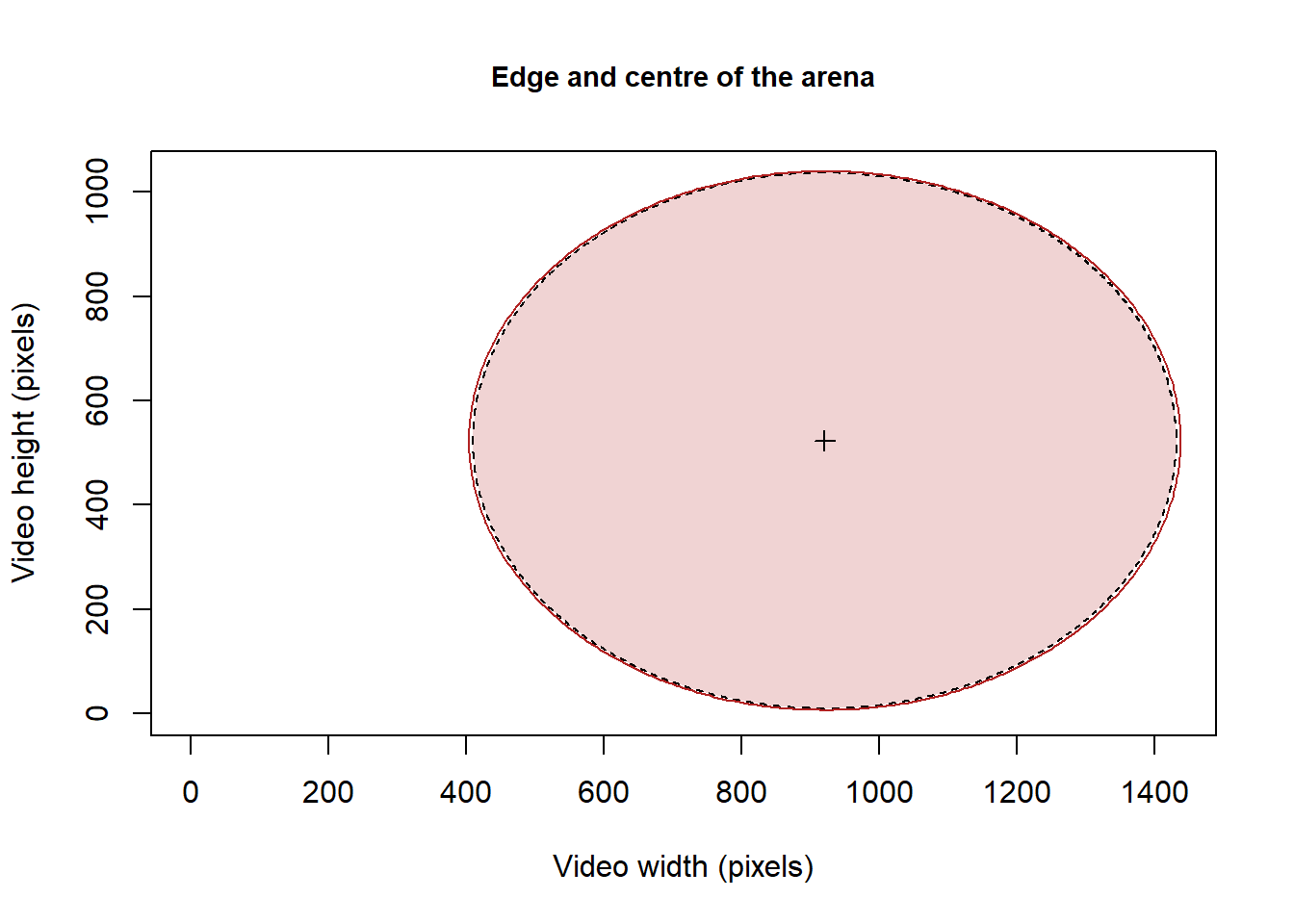
Figure 4: Representation of centre and edge of the arena retrieved from a distance matrix generated using color tresholding in imageJ. The position of the arena edge can be extracted from the distance matrix as the lowest value of distance matrix (i.e., 1) and the centre of the arena as the mean of the edge x and y coordinates.
# here the coordinates of the arena edge are then stored in the ArenaEdge objectHere the distance matrix generated using ImageJ returns decreasing distance from the centre of the arena to the edge.
Accordingly, the lowest value (i.e., 1) corresponds to the edge of the arena (fig. 4, black line). Hence, the use of a distance matrix may be a a good option to retrieve the location of the edge of an arena or any ROI, whatever its shape.
However, in the case of using a classic circular or polygonal arena a simpler approach would consist of generating the expected arena edge using circles() or polygons() and feeding the former with coordinates of the arena center and the radius length (fig. 4, red line).
We can then easily identify whether a particle is detect within or outside the arena by assigning the ROI to each tracklet using the assignROI() and filtering out the tracklets parts detected outside the arena.
## assign The ROI (here the arena) to the particles' positions
trackDat4 <-
  MoveR::analyseTracklets(trackDat.speedfilt[[2]],
                          customFunc = list(
                            Arena = function(x)
                              MoveR::assignROI(
                                x,
                                ROIs = edge,
                                edgeInclude = F,
                                order = T
                              )
                          ))

# draw the tracklet and the arena edges
MoveR::drawTracklets(trackDat4,
                     timeCol = "runTimelinef",
                     add2It = list(graphics::polygon(x = edge$x.pos, y = edge$y.pos)))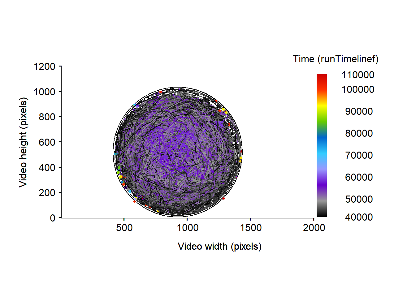
Figure 5: Micro-wasps trajectories over the whole video timeline, expressed in frame. The arena edges are represented by the black circle.
Apparently the amount of artifact detected outside the arena is null or very low (see fig. 5. However, by using assignROI() and excluding the edge some tracklet part are indeed detected outside the arena.
# create the filter to remove particles outside the arena
filter.out <-
  MoveR::filterFunc(
    trackDat4,
    toFilter = "Arena",
    customFunc = function(x)
      x == FALSE
  )

# apply the filter on the data using the frame rate as minimum duration of the tracklets
trackDat.borderfilt <-
  MoveR::filterTracklets(trackDat4,
              filter.out,
              splitCond = TRUE,
              minDur = MoveR::getInfo(trackDat4, "frameR"))
## Warning in MoveR::filterTracklets(trackDat4, filter.out, splitCond = TRUE, : For Tracklet_2:
## All the new tracklets created after filtering are shorter than minDur, no tracklet returned## Warning in MoveR::filterTracklets(trackDat4, filter.out, splitCond = TRUE, : For Tracklet_3724:
## All the new tracklets created after filtering are shorter than minDur, no tracklet returned
# rename the cleaned dataset for further use
trackDat5 <- trackDat.borderfilt[[2]]

# check that the particle detected outside has been removed
## retrieve the ROI assignation before and after filtering
compar <- list(
  before = MoveR::convert2List(trackDat4)[["Arena"]],
  after = MoveR::convert2List(trackDat5)[["Arena"]]
)

## create a count table to determine the amount of tracklets parts that are within and outside the arena
res <- data.frame(matrix(NA, nrow = 2, ncol = 2))
colnames(res) <- unique(compar[[1]])
rownames(res) <- unique(names(compar))
for (i in seq_along(compar)) {
  res[i, "ROI_1"] <- length(grep("\\<ROI_1\\>", compar[[i]]))
  res[i, "FALSE"] <- length(grep("\\<FALSE\\>", compar[[i]]))
}

res
## ROI_1 FALSE
## before 1094821 54
## after 1094821 0Then, as expected the filtering step based the location of the particles inside or outside the arena have removed parts of the tracklets (54 occurrences) detected outside the arena (ROI_1).
# display the information about the filtering process (see ??filterTracklets())
str(trackDat.borderfilt[[1]])
## List of 8
## $ Tracknb_before_filter : int 5803
## $ Tracknb_after_filter : int 5803
## $ Tracknb_after_minDur : num 5801
## $ TotTrackDuration_before_filter: int 1094875
## $ TotTrackDuration_after_filter : int 1094823
## $ TotTrackDuration_after_minDur : int 1094821
## $ %Data_kept_after_filter : num 100
## $ %Data_kept_after_minDur : num 100In addition, according to the summary of the filtering step, the amount of data removed by the filtering is very low (<0.1%), confirming that there is few tracking artifact outside of the arena (fig. 5).
Accordingly, the filter splited only few tracklets in small part resulting in less than 0.1% of data removed because resulting tracklets were shorter than 1 second (25 frames).
While the count table and the summary of the filtering give a general quantitative view of the amount of data removed by the filtering step one may also want to have an idea of the tracklets identity and the spatio-temporal distribution of the removed data. For this we can use drawTracklets() as follow:
# identify the part of the tracklets that are detected outside the arena
trackDat4List <- MoveR::convert2List(trackDat4)
OutTracklets <- unique(trackDat4List[["trackletId"]][which(trackDat4List[["Arena"]] == FALSE)])
OutTracklets
## [1] "Tracklet_2" "Tracklet_3724"
# identify the part of the tracklets that are detected outside the arena
trackDat4List <- MoveR::convert2List(trackDat4)
OutTracklets <- unique(trackDat4List[["trackletId"]][which(trackDat4List[["Arena"]] == FALSE)])
OutTracklets
## [1] "Tracklet_2" "Tracklet_3724"
# plot them
MoveR::drawTracklets(
  trackDat4,
  selTrack = OutTracklets,
  main = ,
  cex.main = 0.9,
  cex.start = 1, # increase the size of the start points of the tracklet (help to locate it, particularly if the particle is still)
  add2It = list(graphics::polygon(x = edge$x.pos, y = edge$y.pos))
)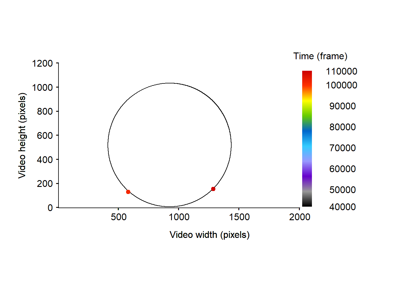
Figure 6: Representation of the particles’ trajectories detected outside the arena before the filtering process removing the moments where the particles are detected outside of the arena.
Here we can see that the tracklets’ part detected outside the arena belong to two tracklets that stayed still over the video-recording (“Tracklet_2” and “Tracklet_3724”). We can thus be confident about the fact that it should be considered as tracking artifacts.
Now we have achieved the filtering of the dataset, one would take a look and eventually save a summary of the filtering procedure.
Filtering/Cleaning summary
Once the filtering/cleaning steps are done, the various filter summaries can be retrieved and easily grouped and eventually saved.
# create a summary of each filter results
FilterSummary <- do.call("cbind",
                         list(
                           data.frame(Infilt = unlist(trackDat.Infilt[[1]])),
                           data.frame(lenfilt = unlist(trackDat.lenfilt[[1]])),
                           data.frame(speedfilt = unlist(trackDat.speedfilt[[1]])),
                           data.frame(outfilt = unlist(trackDat.borderfilt[[1]]))
                         ))

# add cumulative_%Data_kept_after_filter and after_minDur
FilterSummary <- rbind(FilterSummary,
      apply(FilterSummary, 2, FUN = function(x) as.numeric(x[5])/FilterSummary[4,1]*100),
      apply(FilterSummary, 2, FUN = function(x) as.numeric(x[6])/FilterSummary[4,1]*100))
rownames(FilterSummary)[c(9,10)] <- c("cumulative_%Data_kept_after_filter",
                                      "cumulative_%Data_kept_after_minDur")

FilterSummary
## Infilt lenfilt speedfilt
## Tracknb_before_filter 8.800000e+01 6.724000e+03 5.520000e+03
## Tracknb_after_filter 1.655830e+05 1.399700e+04 6.508000e+03
## Tracknb_after_minDur 6.724000e+03 5.520000e+03 5.803000e+03
## TotTrackDuration_before_filter 4.716398e+06 1.177729e+06 1.104334e+06
## TotTrackDuration_after_filter 1.664533e+06 1.133835e+06 1.103235e+06
## TotTrackDuration_after_minDur 1.177729e+06 1.104334e+06 1.094875e+06
## %Data_kept_after_filter 3.529246e+01 9.627300e+01 9.990048e+01
## %Data_kept_after_minDur 2.497094e+01 9.376809e+01 9.914347e+01
## cumulative_%Data_kept_after_filter 3.529246e+01 2.404027e+01 2.339147e+01
## cumulative_%Data_kept_after_minDur 2.497094e+01 2.341478e+01 2.321422e+01
## outfilt
## Tracknb_before_filter 5.803000e+03
## Tracknb_after_filter 5.803000e+03
## Tracknb_after_minDur 5.801000e+03
## TotTrackDuration_before_filter 1.094875e+06
## TotTrackDuration_after_filter 1.094823e+06
## TotTrackDuration_after_minDur 1.094821e+06
## %Data_kept_after_filter 9.999525e+01
## %Data_kept_after_minDur 9.999507e+01
## cumulative_%Data_kept_after_filter 2.321312e+01
## cumulative_%Data_kept_after_minDur 2.321307e+01As previously stated, we can indeed see that the filter based on infinite values have removed a lot of data contrary to the other filters. Also, it seems that the minimum duration of the tracklets set to 25 frames (1 second) is appropriate since it remove a small amount of data.
It is also possible to display a summary of the tracking information of both the initial dataset (i.e., trackDat) and the filtered/cleaned one (trackDat5) using summary() to quickly compare them.
# compute and display a detailed summary of the tracking information before and after cleaning (see ??summary())
Data_Trex_stats_before_filter <-
  summary(trackDat,
                    frameR = MoveR::getInfo(trackDat, "frameR"),
                    scale = MoveR::getInfo(trackDat, "scale"),
                    unit = "cm")
## List of 2
## $ VideoSummary :List of 4
## ..$ videoDuration_f: num 105138
## ..$ videoDuration_s: num 4206
## ..$ frameR : num 25
## ..$ scale : num 0.00242
## $ TrackletSummary:List of 8
## ..$ trackNb : int 88
## ..$ totTrackDuration_f: int 4716398
## ..$ totTrackDuration_s: num 188656
## ..$ totTrackLength_cm : num NaN
## ..$ trackletId : chr [1:88] "434" "435" "436" "437" ...
## ..$ trackDuration_f : int [1:88] 12074 12079 12079 12079 12079 12083 12084 12084 12084 12084 ...
## ..$ trackDuration_s : num [1:88] 483 483 483 483 483 ...
## ..$ trackLength_cm : num [1:88] NaN NaN NaN NaN NaN NaN NaN NaN NaN NaN ...
Data_Trex_stats_after_filter <-
  summary(trackDat5,
                    frameR = MoveR::getInfo(trackDat5, "frameR"),
                    scale = MoveR::getInfo(trackDat5, "scale"),
                    unit = "cm")
## List of 2
## $ VideoSummary :List of 4
## ..$ videoDuration_f: num 105138
## ..$ videoDuration_s: num 4206
## ..$ frameR : num 25
## ..$ scale : num 0.00242
## $ TrackletSummary:List of 8
## ..$ trackNb : int 5801
## ..$ totTrackDuration_f: int 1094821
## ..$ totTrackDuration_s: num 43793
## ..$ totTrackLength_cm : num 7716
## ..$ trackletId : chr [1:5801] "Tracklet_1" "Tracklet_2" "Tracklet_3" "Tracklet_4" ...
## ..$ trackDuration_f : int [1:5801] 138 32 41 60 43 88 46 338 530 255 ...
## ..$ trackDuration_s : num [1:5801] 5.52 1.28 1.64 2.4 1.72 ...
## ..$ trackLength_cm : num [1:5801] 0.059 0.0777 0.0182 0.0261 0.0126 ...By comparing the summary of the tracking information before and after the filtering process, we can see that video characteristics are unchanged.
On the contrary, tracklets are more numerous and shorter after the filtering than before which is not surprising since we have removed biased data and splited the tracklets accordingly.
Both kind of summaries can then be saved as a .csv file using common function such as utils::write.csv() or data.table::fwrite().
Also, the filtered dataset can be saved before using it for further computations.
As such dataset can be large we recommend to use data.table::fwrite() from the data.table package as well as saving the data as .gz archive to save as much disk space as possible (e.g., For this dataset: .csv = 181Mo vs .csv.gz = 62Mo).
# save the cleaned dataset as .csv compressed as .gz
data.table::fwrite(
  MoveR::convert2List(trackDat5),
  paste(paste(dirname(Path2Data[1]), "cleanedData", sep = "/"
  ), "csv", "gz", sep = "."),
  sep = ";",
  dec = ".",
  na = "NA",
)
Now that the filtering/cleaning process is achieved, we can move to data analysis through various metrics computations.
Note, however, that ones would add or replace some of the filters that have been used in this example depending on the model species and the study’ aims. Accordingly, the various function developed in the MoveR package are very flexible and allow the user to specify custom functions to break limits.
For more insight how to use MoveR to run further computation check the next tutorials.
Happy coding.
References
Ion Scotta, M., Margris, L., Sellier, N., Warot, S., Gatti, F., Siccardi, F., Gibert, P., Vercken, E., Ris, N., 2021. Genetic Variability, Population Differentiation, and Correlations for Thermal Tolerance Indices in the Minute Wasp, Trichogramma cacoeciae. Insects 12, 1013. https://doi.org/10.3390/insects12111013
Walter, T., Couzin, I.D., 2021. TRex, a fast multi-animal tracking system with markerless identification, and 2D estimation of posture and visual fields. eLife 10, e64000. https://doi.org/10.7554/eLife.64000