Now that we are familiar with importing and cleaning/filtering raw data from tracking software, we will go deeper by computing various metrics over tracklets and time.
For this example we are selecting the second sample of data available in the MoveR_SampleData github repository. For more detail about this dataset see the introduction of the Clean/Filter Data vignette.
Import sample data from github.
Let’s download the data, import and convert them to a list of tracklets (see the Import Data vignette for detailed procedure).
Here we are avoiding redundancy by using the already cleaned version of the dataset.
# dl the second dataset from the sample data repository
Path2Data <- MoveR::DLsampleData(dataSet = 2, tracker = "TRex")

# Import the sample data
TRexDat <- data.table::fread(
  Path2Data[[3]],
  sep = ";",
  dec = ".")

# convert the data to a list of tracklets - here the data were saved as a varList object (a list of variable) a more simple structure than tracklets
trackDat <- MoveR::convert2Tracklets(TRexDat, by = "trackletId")

# set some useful information
trackDat <- MoveR::setInfo(trackDat, frameR = 25, scale = 1/413.4, imgRes = c(1920, 1080))
Okay! now that the data has been retrieved let’s start computing metric over each tracklet.
Compute metrics over tracklets
While the Clean/Filter Data vignette have already given some hint on the use of analyseTracklets() (i.e., computation of the particles’ speed using speed() and distance to the edge using dist2Edge()) here we are using it more extensively.
For instance, one would compute the following metrics over each tracklet:
the turning angle using
turnAngle()the speed using
speed()- although we already have computed it at the Clean/Filter Data step we need to compute it again to ensure that the values are correct, especially at the start and end of the tracklets because filtering the tracklets may have resulted in spliting them.the distance traveled using
distTraveled()the distance to the edge using
dist2Edge()the “simple” activity computed based on speed and a treshold specified by the user using
activity1()the sinuosity using
sinuosity()the surface explored using
exploredArea()
Note that the distance to the edge of the arena does not need to be computed again since we already did it to remove the moments where the particles were detected outside the arena.
Also it is possible to smooth selected metrics over each tracklet using slidWindow(). For this example we are smoothing the following metrics using a sliding window of 10 frames (Tstep argument):
the mean turning angle and its variance
the mean speed and its variance
the mean distance traveled
the mean distance to the edge
Note that the sinuosity and the surface explored do not need to be smoothed because both functions return a single value for each tracklet (i.e., this value is repeated over the tracklet’s duration).
Before computing the listed metrics, we need to specify some parameters, especially for dist2Edge(), activity1() and exploredArea().
Indeed, to compute the distance from the edges of the arena we need to import the location of the edge (the region of interest - ROI) from a distance matrix using locROI().
Note that generating the distance matrix is an external process that can be achieved using image processing program such as ImageJ.
arenaEdge <- MoveR::locROI(Path2Data[[2]], edgeCrit = 1, xy = 1, order = T)Also, to classify the particles between “active” (1) or “inactive” (0) state, we need to find the speed threshold above which a particle is considered as active and feed the minSpeed argument with it. To do that, we can plot the distribution of particles’ speed and find the valley in the bimodal distribution (fig. 1).
# as specified we need to compute speed over each tracklet
trackDat <-
  MoveR::analyseTracklets(trackDat,
                          customFunc = list(
                            speed = function(x)
                              MoveR::speed(x,
                                           timeCol = "runTimelinef",
                                           scale = 1)))

# plot the distribution of particles' speed
## retrieve the log-transformed speed over all tracklets
speedLog <- log10(MoveR::convert2List(trackDat)$speed)

## computes kernel density estimates of the distribution and plot it
speedLogDens <- data.frame(stats::density(speedLog, na.rm = T)[c(1,2)])
plot(speedLogDens, type = "l")

# find the valley between the two peak of the bimodal distribution using the cardidates package
## if needed install the package install.packages("cardidates")
## identify the peaks of the bimodal distribution and keep only the data between the peaks
peaks <- cardidates::peakwindow(speedLogDens)$peaks$x
speedLogDensReduced <- speedLogDens[-which(speedLogDens$x < peaks[1] | speedLogDens$x > peaks[2]),]

## the valley correspond to the local minimum between the peaks
valley <- speedLogDensReduced$x[which.min(speedLogDensReduced$y)]

## add the peaks and the valley to the plot
abline(v = peaks, col="darkgreen")
abline(v = valley, col="firebrick")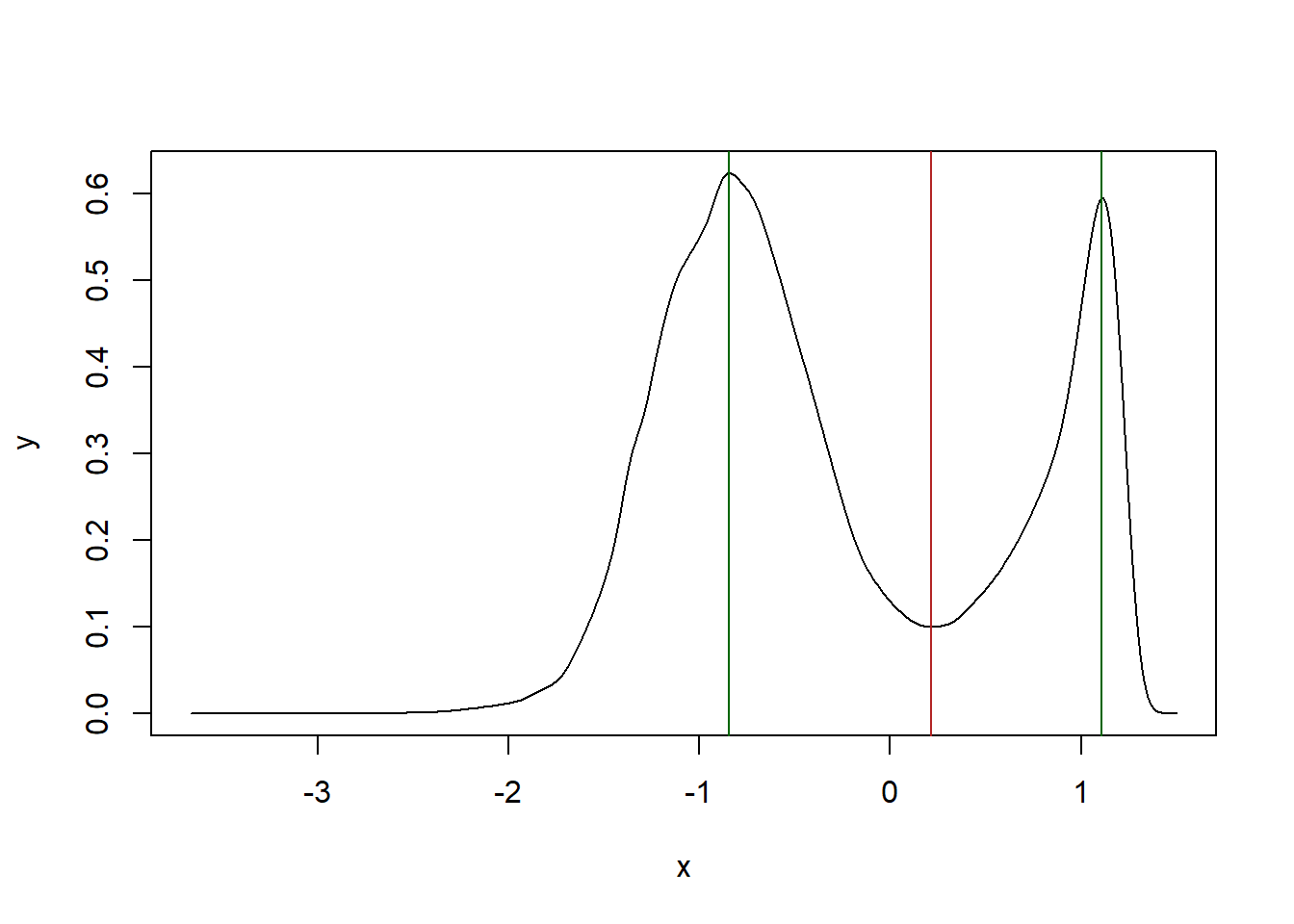
Figure 1: kernel density estimate of the particles’ speed. The bimodal distribution allow to classify activity states between active and inactive based on 1 dimension. Peaks of the distribution are represented by the green vertical lines while the valley corresponding to the treshold above which particles are considered as active is represented by the red vertical line.
## as the the data were log-transformed we need to back-transform the value of the valley to find the threshold to determine the activity state

activTresh <- 10^valley
activTresh
## [1] 1.648978We have found the threshold above which the particles are considered as active.
Now need to identify the diameter of the typical surface a particle can “explore” around its position to determine the surface explored over each tracklet. To do that, we need some knowledge about the model species.
In the case of Trichogramma, Wajnberg and Colazza (1998) reported that the perception distance (i.e., reaction distance) of an individual is about 4 mm. Accordingly, we can infer that an individual should explore a surrounding surface of 16 mm2. The diameter of such a cell is hence 8 mm or 331 pixels which corresponds to the binRad argument.
diamSurf <- 0.8 / MoveR::getInfo(trackDat, "scale")Now we have everything that is needed to run the computation of the desired metrics the first step consist in specifying a list of custom functions as follow:
# Specify the batch of function to pass to the analyseTracklet function for metric computation over each tracklet
customFuncList = list(
  ## compute
  ### turning angles
  turnAngle = function(x)
    MoveR::turnAngle(
      x,
      unit = "radians",
      timeCol = "runTimelinef",
      scale = 1
    ),
  ###distance traveled
  distTraveled = function(x)
    MoveR::distTraveled(x,
                        step = 1),
  ###distance to the edge of the arena based on the form of the arena (here circular)
  dist2Edge = function(x)
    MoveR::dist2Edge(x,
                     edge = arenaEdge,
                     customFunc = "CircularArena"),
  ###activity
  activity1 = function(x)
    MoveR::activity1(x,
                     speedCol = "speed",
                     minSpeed = activTresh),
  ###sinuosity
  sinuosity = function(x)
    MoveR::sinuosity(x,
                     timeCol = "runTimelinef",
                     scale = 1),
  ### surface explored
  explorArea = function(x)
    MoveR::exploredArea(
      x,
      binRad = diamSurf,
      timeCol = "runTimelinef",
      scale = 1,
      graph = F
    ),
  ## Smooth
  ### turning angles
  slideMeanAngle = function (y)
    MoveR::slidWindow(y$turnAngle,
                   Tstep = 10,
                   statistic = "mean",
                   na.rm = T),
  ### turning angles variance
  slideVarAngle = function (y)
    MoveR::slidWindow(circular::circular(y$turnAngle,
                                      type = "angle",
                                      units = "radians"),
                   Tstep = 10,
                   statistic = "circular.var",
                   na.rm = T),
  ### speed
  slideMeanSpeed = function (y)
    MoveR::slidWindow(y$speed,
                   Tstep = 10,
                   statistic = "mean",
                   na.rm = T),
  ### speed variance
  slideVarSpeed = function (y)
    MoveR::slidWindow(y$speed,
                   Tstep = 10,
                   statistic = "var",
                   na.rm = T),
  ### smooth traveled distance
  slideMeanTraveledDist = function (y)
    MoveR::slidWindow(y$distTraveled,
                   Tstep = 10,
                   statistic = "mean",
                   na.rm = T),
  ### distance to the edge
  slideMeanDist2Edge = function (y)
    MoveR::slidWindow(y$dist2Edge,
                   Tstep = 10,
                   statistic = "mean",
                   na.rm = T)
)
Note that naming each element (function) of the list ensure that the output of the computation is properly named when appended to the data. In case list elements are unnamed, the analyseTracklets() look for a generic name within the specified customFunc.
For instance, for turnAngle(x, TimeCol = "runTimelinef", unit = "radians"), the function can retrieve turnAngle but the result can be unexpected in case of more complex function structure such as for circular::var(circular::circular(x$turnAngle, type = "angle", units = "radians"), na.rm = T), here the function will extract circular::var.
Everything is ok, let’s start the computation using analyseTracklets()
trackDat2 <-
  MoveR::analyseTracklets(trackDat,
                          customFunc = customFuncList)

head(trackDat2[[1]], 20)
## maj.ax angle min.ax x.pos y.pos identity frame runTimelinef
## 1 16.55498 -0.04423860 NA 639.2191 165.7905 434 103180 103180
## 2 16.74520 -0.04471057 NA 639.2343 165.8378 434 103181 103181
## 3 16.76947 -0.09136654 NA 639.1810 165.7524 434 103182 103182
## 4 16.11969 -3.06878567 NA 638.9434 165.8585 434 103183 103183
## 5 16.36526 -0.13061114 NA 639.1569 165.8431 434 103184 103184
## 6 16.36526 -0.13061114 NA 639.1942 165.8738 434 103185 103185
## 7 15.62286 3.08025122 NA 639.1310 166.2738 434 103186 103186
## 8 15.98815 3.13638091 NA 639.3047 166.0190 434 103187 103187
## 9 16.57985 -0.04749756 NA 639.3143 165.9238 434 103188 103188
## 10 15.84952 -0.07241549 NA 639.3535 165.8384 434 103189 103189
## 11 16.10183 -0.06872617 NA 639.1124 166.3483 434 103190 103190
## 12 16.19552 -0.06412730 NA 639.2843 165.8922 434 103191 103191
## 13 16.44985 -0.04795182 NA 639.2816 165.8252 434 103192 103192
## 14 16.30862 -0.03188454 NA 639.3593 165.8932 434 103193 103193
## 15 16.25080 -0.04683051 NA 639.2330 165.8544 434 103194 103194
## 16 16.44985 -0.04795182 NA 639.2816 165.8252 434 103195 103195
## 17 16.47299 -0.04132291 NA 639.3619 165.8190 434 103196 103196
## 18 16.25080 -0.04683051 NA 639.2692 165.8846 434 103197 103197
## 19 16.25080 -0.04683051 NA 639.2330 165.8544 434 103198 103198
## 20 16.47299 -0.04132291 NA 639.3019 165.8491 434 103199 103199
## runTimelineS Measured_Temp_Deg_C indLengthcm speed dist2Edge trackletId
## 1 4127.20 35.7 0.04004591 NA -56.74821 Tracklet_1
## 2 4127.24 35.7 0.04050604 0.04974185 -56.79482 Tracklet_1
## 3 4127.28 35.7 0.04056475 0.10071409 -56.69472 Tracklet_1
## 4 4127.32 35.7 0.03899297 0.26017052 -56.63100 Tracklet_1
## 5 4127.36 35.7 0.03958699 0.21399122 -56.75109 Tracklet_1
## 6 4127.40 35.7 0.03958699 0.04826507 -56.79823 Tracklet_1
## 7 4127.44 35.7 0.03779116 0.40498167 -57.07324 Tracklet_1
## 8 4127.48 35.7 0.03867476 0.30837970 -56.98078 Tracklet_1
## 9 4127.52 35.7 0.04010607 0.09570492 -56.91187 Tracklet_1
## 10 4127.56 35.7 0.03833944 0.09401691 -56.86904 Tracklet_1
## 11 4127.60 35.7 0.03894977 0.56407927 -57.12019 Tracklet_1
## 12 4127.64 35.7 0.03917639 0.48748878 -56.86846 Tracklet_1
## 13 4127.68 35.7 0.03979160 0.06696614 -56.81419 Tracklet_1
## 14 4127.72 35.7 0.03944999 0.10322724 -56.91566 Tracklet_1
## 15 4127.76 35.7 0.03931012 0.13205952 -56.80705 Tracklet_1
## 16 4127.80 35.7 0.03979160 0.05659485 -56.81419 Tracklet_1
## 17 4127.84 35.7 0.03984757 0.08056082 -56.85902 Tracklet_1
## 18 4127.88 35.7 0.03931012 0.11350467 -56.85320 Tracklet_1
## 19 4127.92 35.7 0.03931012 0.04716597 -56.80705 Tracklet_1
## 20 4127.96 35.7 0.03984757 0.06905213 -56.84548 Tracklet_1
## turnAngle distTraveled activity1 sinuosity explorArea slideMeanAngle
## 1 NA 0.04974185 NA 4.253483 94722.15 NA
## 2 2.8945991 0.10071409 0 4.253483 94722.15 NA
## 3 -1.4333993 0.26017052 0 4.253483 94722.15 NA
## 4 -2.7932937 0.21399122 0 4.253483 94722.15 NA
## 5 0.7595711 0.04826507 0 4.253483 94722.15 -0.6145500
## 6 1.0396458 0.40498167 0 4.253483 94722.15 -0.2470643
## 7 -2.6996207 0.30837970 0 4.253483 94722.15 -0.5766720
## 8 -0.4989445 0.09570492 0 4.253483 94722.15 -0.2002835
## 9 0.3309640 0.09401691 0 4.253483 94722.15 0.3511861
## 10 -3.1304721 0.56407927 0 4.253483 94722.15 0.5054759
## 11 3.0603075 0.48748878 0 4.253483 94722.15 0.4478788
## 12 -0.4014782 0.06696614 0 4.253483 94722.15 0.9781119
## 13 2.3304855 0.10322724 0 4.253483 94722.15 1.1591985
## 14 2.7214030 0.13205952 0 4.253483 94722.15 1.3629575
## 15 2.3024685 0.05659485 0 4.253483 94722.15 1.7512710
## 16 0.4636754 0.08056082 0 4.253483 94722.15 1.7192587
## 17 2.6027098 0.11350467 0 4.253483 94722.15 2.0475425
## 18 1.3119219 0.04716597 0 4.253483 94722.15 1.5778359
## 19 2.3685536 0.06905213 0 4.253483 94722.15 1.1360680
## 20 0.7526626 0.11835048 0 4.253483 94722.15 1.2199804
## slideVarAngle slideMeanSpeed slideVarSpeed slideMeanTraveledDist
## 1 NA NA NA NA
## 2 NA NA NA NA
## 3 NA NA NA NA
## 4 NA NA NA NA
## 5 0.9295268 0.17510733 0.0161964567 0.21400452
## 6 0.8381583 0.21400452 0.0295267675 0.25777921
## 7 0.9264664 0.25777921 0.0327100097 0.25440442
## 8 0.8828520 0.25440442 0.0340018192 0.23871009
## 9 0.8142052 0.23871009 0.0362638385 0.23051692
## 10 0.7342879 0.23051692 0.0373851765 0.23134990
## 11 0.7909803 0.23134990 0.0370547556 0.19890781
## 12 0.7208400 0.19890781 0.0350619184 0.17942031
## 13 0.5647072 0.17942031 0.0341188046 0.17456642
## 14 0.4369973 0.17456642 0.0352573980 0.17206994
## 15 0.4714105 0.17206994 0.0357665888 0.12749706
## 16 0.4454715 0.12749706 0.0168051498 0.09016746
## 17 0.3009847 0.09016746 0.0008771468 0.09096670
## 18 0.4129182 0.09096670 0.0008423269 0.09243493
## 19 0.5688037 0.09243493 0.0009038864 0.09400368
## 20 0.5897723 0.09400368 0.0010666324 0.10311890
## slideMeanDist2Edge
## 1 NA
## 2 NA
## 3 NA
## 4 NA
## 5 -56.82530
## 6 -56.86250
## 7 -56.86986
## 8 -56.88181
## 9 -56.91028
## 10 -56.91587
## 11 -56.91747
## 12 -56.89605
## 13 -56.88329
## 14 -56.87281
## 15 -56.87045
## 16 -56.85451
## 17 -56.85451
## 18 -56.86466
## 19 -56.85294
## 20 -56.85560Great! as displayed above for the first tracklet, the desired metrics and the smoothed one has been added to the dataset.
Note that sinuosity and explorArea return an unique value, in this case, the value is repeated over the whole tracklet. Also note that as we choose a step of 10 time units (here frames) for each sliding window, the first and last 5 values of the computed metrics return NA.
To summarize, it is easy to run relatively intensive computation on a large set of tracklets and smooth the resulting metrics over each tracklet. While for this example, we have combined analyseTracklets(), slidWindow() and various modulus (e.g., speed(), sinuosity(), turnAngle()), analyseTracklets() is flexible enough to accept any computation specified by the user within the “customFunc” argument.
To go further, while we have identified activity states (i.e., active vs inactive) based on 1 dimension using active1(), one may also perform activity states classification trough non-hierarchical clustering in 2 dimensions using activity2().
activity states: 2 dimensions non-hierarchical clustering
The MoveR package allow to use density based clustering (Henning 2020; Ester et al., 1996) on two a dimensions array to classify particles’ between active and inactive states.
For this purpose, we are using activity2() and the previously smoothed speed (log-transformed) and turning angle variance as dimensions to performed non-hierarchical clustering as follow:
# use density based clustering to classify actives and inactives states in a 2 dimension array (here the smoothed speed (log) and the angle variance)

trackDat3 <-
  MoveR::activity2(
    trackDat2,
    var1 = "slideMeanSpeed",
    var2 = "slideVarAngle",
    var1T = log10,
    nbins = 100,
    eps = 0.15,
    minPts = 5
  )
## [1] "Clusters identified !"
head(trackDat3[[1]], 20)## maj.ax angle min.ax x.pos y.pos identity frame runTimelinef
## 1 16.55498 -0.04423860 NA 639.2191 165.7905 434 103180 103180
## 2 16.74520 -0.04471057 NA 639.2343 165.8378 434 103181 103181
## 3 16.76947 -0.09136654 NA 639.1810 165.7524 434 103182 103182
## 4 16.11969 -3.06878567 NA 638.9434 165.8585 434 103183 103183
## 5 16.36526 -0.13061114 NA 639.1569 165.8431 434 103184 103184
## 6 16.36526 -0.13061114 NA 639.1942 165.8738 434 103185 103185
## 7 15.62286 3.08025122 NA 639.1310 166.2738 434 103186 103186
## 8 15.98815 3.13638091 NA 639.3047 166.0190 434 103187 103187
## 9 16.57985 -0.04749756 NA 639.3143 165.9238 434 103188 103188
## 10 15.84952 -0.07241549 NA 639.3535 165.8384 434 103189 103189
## 11 16.10183 -0.06872617 NA 639.1124 166.3483 434 103190 103190
## 12 16.19552 -0.06412730 NA 639.2843 165.8922 434 103191 103191
## 13 16.44985 -0.04795182 NA 639.2816 165.8252 434 103192 103192
## 14 16.30862 -0.03188454 NA 639.3593 165.8932 434 103193 103193
## 15 16.25080 -0.04683051 NA 639.2330 165.8544 434 103194 103194
## 16 16.44985 -0.04795182 NA 639.2816 165.8252 434 103195 103195
## 17 16.47299 -0.04132291 NA 639.3619 165.8190 434 103196 103196
## 18 16.25080 -0.04683051 NA 639.2692 165.8846 434 103197 103197
## 19 16.25080 -0.04683051 NA 639.2330 165.8544 434 103198 103198
## 20 16.47299 -0.04132291 NA 639.3019 165.8491 434 103199 103199
## runTimelineS Measured_Temp_Deg_C indLengthcm speed dist2Edge trackletId
## 1 4127.20 35.7 0.04004591 NA -56.74821 Tracklet_1
## 2 4127.24 35.7 0.04050604 0.04974185 -56.79482 Tracklet_1
## 3 4127.28 35.7 0.04056475 0.10071409 -56.69472 Tracklet_1
## 4 4127.32 35.7 0.03899297 0.26017052 -56.63100 Tracklet_1
## 5 4127.36 35.7 0.03958699 0.21399122 -56.75109 Tracklet_1
## 6 4127.40 35.7 0.03958699 0.04826507 -56.79823 Tracklet_1
## 7 4127.44 35.7 0.03779116 0.40498167 -57.07324 Tracklet_1
## 8 4127.48 35.7 0.03867476 0.30837970 -56.98078 Tracklet_1
## 9 4127.52 35.7 0.04010607 0.09570492 -56.91187 Tracklet_1
## 10 4127.56 35.7 0.03833944 0.09401691 -56.86904 Tracklet_1
## 11 4127.60 35.7 0.03894977 0.56407927 -57.12019 Tracklet_1
## 12 4127.64 35.7 0.03917639 0.48748878 -56.86846 Tracklet_1
## 13 4127.68 35.7 0.03979160 0.06696614 -56.81419 Tracklet_1
## 14 4127.72 35.7 0.03944999 0.10322724 -56.91566 Tracklet_1
## 15 4127.76 35.7 0.03931012 0.13205952 -56.80705 Tracklet_1
## 16 4127.80 35.7 0.03979160 0.05659485 -56.81419 Tracklet_1
## 17 4127.84 35.7 0.03984757 0.08056082 -56.85902 Tracklet_1
## 18 4127.88 35.7 0.03931012 0.11350467 -56.85320 Tracklet_1
## 19 4127.92 35.7 0.03931012 0.04716597 -56.80705 Tracklet_1
## 20 4127.96 35.7 0.03984757 0.06905213 -56.84548 Tracklet_1
## turnAngle distTraveled activity1 sinuosity explorArea slideMeanAngle
## 1 NA 0.04974185 NA 4.253483 94722.15 NA
## 2 2.8945991 0.10071409 0 4.253483 94722.15 NA
## 3 -1.4333993 0.26017052 0 4.253483 94722.15 NA
## 4 -2.7932937 0.21399122 0 4.253483 94722.15 NA
## 5 0.7595711 0.04826507 0 4.253483 94722.15 -0.6145500
## 6 1.0396458 0.40498167 0 4.253483 94722.15 -0.2470643
## 7 -2.6996207 0.30837970 0 4.253483 94722.15 -0.5766720
## 8 -0.4989445 0.09570492 0 4.253483 94722.15 -0.2002835
## 9 0.3309640 0.09401691 0 4.253483 94722.15 0.3511861
## 10 -3.1304721 0.56407927 0 4.253483 94722.15 0.5054759
## 11 3.0603075 0.48748878 0 4.253483 94722.15 0.4478788
## 12 -0.4014782 0.06696614 0 4.253483 94722.15 0.9781119
## 13 2.3304855 0.10322724 0 4.253483 94722.15 1.1591985
## 14 2.7214030 0.13205952 0 4.253483 94722.15 1.3629575
## 15 2.3024685 0.05659485 0 4.253483 94722.15 1.7512710
## 16 0.4636754 0.08056082 0 4.253483 94722.15 1.7192587
## 17 2.6027098 0.11350467 0 4.253483 94722.15 2.0475425
## 18 1.3119219 0.04716597 0 4.253483 94722.15 1.5778359
## 19 2.3685536 0.06905213 0 4.253483 94722.15 1.1360680
## 20 0.7526626 0.11835048 0 4.253483 94722.15 1.2199804
## slideVarAngle slideMeanSpeed slideVarSpeed slideMeanTraveledDist
## 1 NA NA NA NA
## 2 NA NA NA NA
## 3 NA NA NA NA
## 4 NA NA NA NA
## 5 0.9295268 0.17510733 0.0161964567 0.21400452
## 6 0.8381583 0.21400452 0.0295267675 0.25777921
## 7 0.9264664 0.25777921 0.0327100097 0.25440442
## 8 0.8828520 0.25440442 0.0340018192 0.23871009
## 9 0.8142052 0.23871009 0.0362638385 0.23051692
## 10 0.7342879 0.23051692 0.0373851765 0.23134990
## 11 0.7909803 0.23134990 0.0370547556 0.19890781
## 12 0.7208400 0.19890781 0.0350619184 0.17942031
## 13 0.5647072 0.17942031 0.0341188046 0.17456642
## 14 0.4369973 0.17456642 0.0352573980 0.17206994
## 15 0.4714105 0.17206994 0.0357665888 0.12749706
## 16 0.4454715 0.12749706 0.0168051498 0.09016746
## 17 0.3009847 0.09016746 0.0008771468 0.09096670
## 18 0.4129182 0.09096670 0.0008423269 0.09243493
## 19 0.5688037 0.09243493 0.0009038864 0.09400368
## 20 0.5897723 0.09400368 0.0010666324 0.10311890
## slideMeanDist2Edge activity2
## 1 NA NA
## 2 NA NA
## 3 NA NA
## 4 NA NA
## 5 -56.82530 0
## 6 -56.86250 0
## 7 -56.86986 0
## 8 -56.88181 0
## 9 -56.91028 0
## 10 -56.91587 0
## 11 -56.91747 0
## 12 -56.89605 0
## 13 -56.88329 0
## 14 -56.87281 0
## 15 -56.87045 0
## 16 -56.85451 0
## 17 -56.85451 0
## 18 -56.86466 0
## 19 -56.85294 0
## 20 -56.85560 0As expected, a new column (activity2) containing particles’ activity states, coded as binary value (1 and 0 for active and inactive state, respectively) is added to each tracklet.
Also, using countMat() it is possible to build the matrix of count in the two dimensions array used to classify particles’ between active and inactive states and then build a 3D plot (e.g., using plotly) showing the distribution of active and inactive states within the specified space (here, smoothed speed (log-transformed) and turning angle variance) (see fig. 2).
 # compute the count matrix in the 2d space with the same parameter than activity2 function
 trackDatL <- MoveR::convert2List(trackDat3)
 outP <- MoveR::countMat(x = log10(trackDatL[["slideMeanSpeed"]]),
                  y = trackDatL[["slideVarAngle"]],
                  groups = trackDatL[["activity2"]],
                  nbins = 100,
                  output = "matrix")

 # retrieve max and min value of sqrt-transformed count over the groups for plotting
 maxVal <- max(unlist(lapply(outP, function(z) max(sqrt(z)))))
 minVal <- min(unlist(lapply(outP, function(z) min(sqrt(z)))))

 # draw the plot using plotly R package (3d interactive plot)
 fig <- plotly::plot_ly(x=~colnames(outP[[1]]), y=~rownames(outP[[1]]), contours = list(
   z = list(
     show = TRUE,
     start = round(minVal,-2),
     project = list(z = TRUE),
     end = round(maxVal,-2),
     size = max(maxVal) / 10,
     color = "white"
   )
 ))
 # add inactive layer
 fig <- plotly::add_surface(
   p = fig,
   z = sqrt(outP[[1]]),
   opacity = 0.8,
   colorscale = "Hot",
   cmin = min(sqrt(outP[[1]])),
   cmax = max(sqrt(outP[[1]])),
   colorbar = list(title = "inactive\ncounts (sqrt)")
 )
 # add active layer
 fig <- plotly::add_surface(
   p = fig,
   z = sqrt(outP[[2]]),
   opacity = 1,
   colorscale = list(
     c(0, 0.25, 1),
     c("rgb(20,20,20)", "rgb(58,139,44)", "rgb(234,239,226)")
   ),
   colorbar = list(title = "active\ncounts (sqrt)")
 )
 fig <- plotly::layout(
   fig,
   title = '3D density plot of activity states',
   scene1 = list(
     xaxis = list(title = "Speed (log10)"),
     yaxis = list(title = "Angle variance"),
     zaxis = list(title = "counts (sqrt)")
   )
 )
 fig
Figure 2: 3d density map of the active and inactive states according to the non-hierarchical classification (density based clustering) performed on smoothed particles speed (log-transformed) and turning angle variance. here the distribution of active and inactive state are represented as a gradient of dark-green to white and dark-red to white according to the increasing number of counts.
This plot may be helpful as diagnostic plot to check the distribution of the data making the two clusters and to check whether the clusters has been identified in an expected way. The count matrix can also be computed before using activity2() to check for global distribution of the count in the specified 2d space.
Indeed, note that to identify the clusters we assume that the distribution of inactive states follow a Gaussian (i.e., normal) distribution within the 2 dimensions space.
The activity state lying within the 95% confidence interval ellipsis of the distribution as well as those that hold values below the major radius of the ellipsis on the x axis and below the minor radius on the y axis are considered as inactive (0) while the remaining one are considered as active (1).
Now we have identified activity states according to both 1d (activity1()) and 2d (activity2()) methods, we can compare the global proportion of both active and inactive state returned by the two functions (see fig. 3 below).
# compare the amount of active and inactive state between activity1() and activity2() functions
par(mfrow=c(1,2))
for (i in c(1:2)) {
  ## compute the proportion of active and inactive states resulting from the activity1 and activity2 functions
  act <- length(which(trackDatL[[paste0("activity", i)]] == 1)) / length(trackDatL[[paste0("activity", i)]][-c(which(is.na(trackDatL[[paste0("activity", i)]])))]) * 100
  inact <- length(which(trackDatL[[paste0("activity", i)]] == 0)) / length(trackDatL[[paste0("activity", i)]][-c(which(is.na(trackDatL[[paste0("activity", i)]])))]) * 100
  ## pie chart of behavioral state proportion for both results
  pie(
  main = paste0("Proportion of active vs. inactive states\nfor activity", i, "()"),
  cex.main = 0.7,
  c(act, inact),
  labels = paste(round(
    data.frame(active = act,
               inactive = inact),
    digits = 2
  ), "%", sep = ""),
  col = c("#99CC66", "#993333")
)
legend(
  .2,
  1.5,
  c("active", "inactive"),
  cex = 0.8,
  fill = c("#99CC66", "#993333")
)
}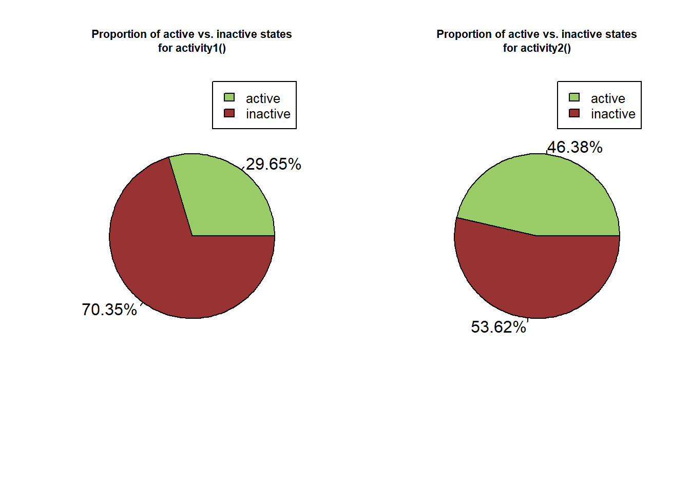
Figure 3: Pie chart representing the proportion of active (green) and inactive (red) state over the whole dataset computed using activity1 (A) and activity2 (B) functions.
Here we can see that the activity1() returns about 2% less active state than activity2() while it seems relatively low, activity2() identify the inactive state more precisely allowing to consider particles that move slowly as active.
Indeed, the general idea behind this kind of activity classification is that the more particle speed increase, the more the trajectory of the particle is straight, although it depend on the model species studied. One can thus choose the classification method to use according to its own system.
Global exploration pattern
While we have already computed the surface explored over each tracklet using exploredArea() combined with analyseTracklets(), one would also compute the total surface explored over the whole dataset and quickly check if the particles’ displacements are homogeneously distributed in space (graph = TRUE).
Note that exploredArea also allow to save the heatmap with or without displaying it by specifying a saving function or a logical value (TRUE) in the saveGraph argument.
# Total surface explored
Totexplored <- MoveR::exploredArea(
  trackDat3,
  binRad = diamSurf,
  timeCol = "runTimelinef",
  scale = 1,
  graph = T
)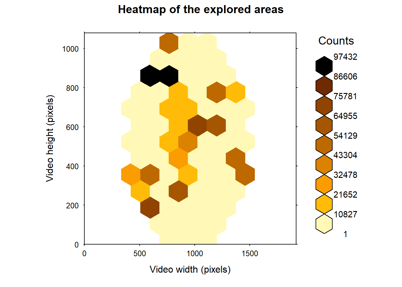
Figure 4: Heatmap of the area visited by the particles. Here we used the reaction distance of Trichogramma according to Wajnberg and Colazza (1998) to infer the diameter of the area an individual can perceive (about 8 mm or 330 pixels).
According to the fig. 4, we can see that the particles have, to a certain extent, visited the arena homogeneously but seems to move further on the upper left corner of the arena. Also, the total surface explored by the particle reached 1894443 pixels2.
To further investigate particular movement patterns across various areas the manage ROI set of functions, including circles(), polygons(), locROI and assignROI, allows to play with the specification of some ROI and then identify movement patterns across area using IdStateSeq().
Sociability index: ANND function
While MoveR does not focus on the study of interaction among particles, we have implemented the possibility to compute the Average Nearest Neighbor Distance (ANND) among particles. The ANND is commonly viewed as an index of sociability in gregarious groups of individuals.
Hence, using ANND() one can compute the Average Nearest Neighbor distance across all particles and time unit. In addition , the function allow to perform a bootstrap over time unit to compute studentize 95% confidence interval around the ANND.
For this example, we are computing the ANND and studentize 95% confidence interval every 20 seconds (i.e., 20 seconds * 25 frames) over 500 bootstrap sampling.
# compute the ANND and studentize 95% confidence interval (bootstrap)
ANNDRes <- MoveR::ANND(
    trackDat3,
    timeCol = "runTimelinef",
    sampling = 20 * 25,
    scale = 1,
    bootn = 500
)

# Retrieve the results and add the timeline of the temperature values to the dataset
ANNDResPlot <- merge(ANNDRes$ANND, trackDatL[c(8,10)], by = "runTimelinef")

# import a custom function to plot the results
source("https://raw.githubusercontent.com/qpetitjean/TrichoG_Thermal_Biology/main/RScripts/Strains_plotFunc.r")

# plot the ANND and studentize 95% confidence interval as an envelope as well as the number of detection over the experiment.
strains_plot(
    finalDatList = trackDatL,
    smoothDf = ANNDResPlot,
    TempAxis = "y",
    TempCol = "Measured_Temp_Deg_C",
    TempScale = c(35,45,2),
    TimeCol = "runTimelinef",
    TimeLimit = c((25*60*25), (70*60*25)),
    nbrIndcounted = 24,
    IC = list(ANNDmean = ANNDResPlot),
    variables = "ANNDmean",
    colvariable = c("#D3139F"),
    scaleVariable = list(c(0,300)),
    Lab = "ANND (pixels)",
    cex.lab = 1,
    xTick = 5,
    InnerSpace = 0.51)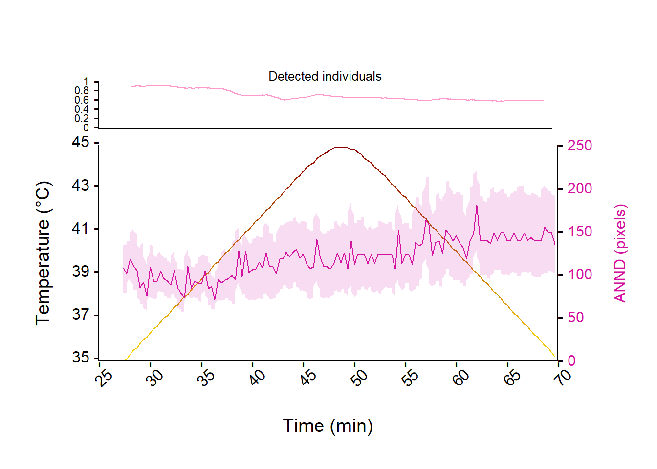
Figure 5: Evolution of the Average Nearest Neighbor Distance (ANND, purple line) and studentize 95% confidence interval among Trichogramma individuals over time and temperature ramp (from 35°C to 45°C and back to 35°C, yellow to red line) expressed in pixels. The upper panel represent the evolution of the number of detected individuals relative to the true number of individual introduced in the arena (i.e., 24) over the experiment.
According to the fig. 5, the ANND is relatively steady over the temperature ramp, although it tend to increase a bit.
Also, we can see on the upper panel that the relative number of detected individual is quite good with about 100% of detection at the start of the experiment and slightly decrease over time to reach about 65%.
The decrease of the amount of detection is mainly due to the fact that over 45℃ most of the individual stop any motion, probably because they died. But further investigation on other traits may shed the light about what is going on here.
Temporal trends
Indeed, while we have previously computed several metrics over each tracklet, we need to investigate how these metrics might be altered over time and hence over the temperature ramp.
To do that, we first should specify a list of custom function to feed temporalTrend(). Here we are using some of the previously computed metrics but one can implement any other metrics and subsequent computation (e.g., mean, var).
For instance,
the mean sinuosity over time
the mean speed of active individual only over time
the mean speed of all individual over time
the mean activity over time (using results of
activity2())the mean surface explored over time
the mean distance to the edge over time
the mean distance traveled over time.
Note that temporalTrend() allow to analyse only specific part of the timeline by specifying the Tinterval argument. More importantly, and as tracklets might present different length, the function allow to weighed the results of the custom functions according to the tracklet length of the tracklets by using the wtd argument.
As the results of the computation are smoothed over time, the sampling and Tstep arguments should be specified to define the sampling step (i.e., the resolution) use for the computation and the size of the sliding window used for smoothing, respectively.
Here, we are using a sampling step of 20 seconds (20 seconds * 25 fps) and a sliding window of 1.5 minutes (90 seconds * 25 fps)
# specify a list of custom function to smooth the existing metrics over time
customFuncList <- list(
  # smooth sinuosity over time
  sinuosity =
    function(x) {
      mean(x$sinuosity, na.rm = T)
    },
  # smooth speed over time for active states only
  speed_active =
    function(x) {
      ifelse(nrow(x[which(!is.na(x$activity2) &
                            x$activity2 == 1),]) == 0, NA,
             mean(x$slideMeanSpeed[which(!is.na(x$activity2) &
                                           x$activity2 == 1)], na.rm = T))
    },
  # smooth speed over time whatever the states
  speed_all =
    function(x) {
      mean(x$slideMeanSpeed, na.rm = T)
    },
  # smooth activity states over time
  activity =
    function(x) {
      if (nrow(x[!is.na(x$activity2),]) == 0) {
        NA
      } else {
        nrow(x[!is.na(x$activity2) &
                 x$activity2 == 1,]) / nrow(x[!is.na(x$activity2),])
      }
    },
  # smooth the exploration over time
  explorArea =
    function(x) {
      mean(x$explorArea, na.rm = T)
    },
  # smooth the distance to the edge whatever the states over time
  Dist2Edge =
    function(x) {
      mean(x$slideMeanDist2Edge, na.rm = T)
    },
  # smooth the distance traveled whatever the states over time
  TraveledDist =
    function(x) {
      mean(x$slideMeanTraveledDist, na.rm = T)
    }
)

# compute the smoothed metrics over time
TemporalRes_wtd <- MoveR::temporalTrend(
  trackDat3,
  timeCol = "runTimelinef",
  customFunc = customFuncList,
  Tstep = 90 * 25,
  sampling = 20 * 25,
  wtd = TRUE
)

# plot the result
par(mfrow = c(2, 4))
for (p in seq_along(TemporalRes_wtd)) {
  plot(
    NULL,
    ylim = c(round(
      min(TemporalRes_wtd[[p]][, 1], na.rm = T),
      digits = 1
    ),
    round(
      max(TemporalRes_wtd[[p]][, 1], na.rm = T),
      digits = 1
    )),
    xlim = c(
      min(TemporalRes_wtd[[p]]$runTimelinef, na.rm = T),
      max(TemporalRes_wtd[[p]]$runTimelinef, na.rm = T)
    ),
    main = names(TemporalRes_wtd)[p],
    ylab = names(TemporalRes_wtd)[p],
    xlab = "Time (frames)"
  )
  lines(TemporalRes_wtd[[p]][, 1] ~ TemporalRes_wtd[[p]]$runTimelinef , col = "darkred")
}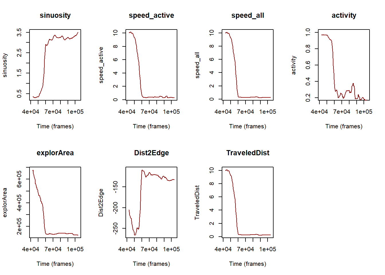
Figure 6: Evolution of the various metrics (sinuosity, speed for active state, speed including all activity states, activity, surface explored, distance to the edge of the arena and distance traveled by the individuals) over the experiment timeline expressed in frames.
Here we are, after a quick look at this panel of plots (fig. 6) it seems that there is a common trend across all metrics with a tipping point marking either a drastic decrease or increase depending on the considered metric.
More particularly, there is a drop on speed (whatever which metric is considered), activity, surface explored, distance to the edge (here the more the value is negative, the more the individuals far from the edge) and distance traveled while there is an increase of sinuosity.
While this observation is encouraging, we need to check whether the variability around the computed values are small enough too support it. This could then help us to find the tipping point (i.e., temperature threshold) which hampered Trichogramma’s movements.
Accordingly, let’s start computing studentized 95% confidence interval using temporalTrend():
TemporalResBOOT_wtd <-
  MoveR::temporalBoot(
    trackDat = trackDat3,
    timeCol = "runTimelinef",
    customFunc = customFuncList,
    Tstep = 90 * 25,
    sampling = 20 * 25,
    bootn = 500,
    wtd = TRUE
  )

# retrieve the CI from the output of temporalBoot
boot.ci <- TemporalResBOOT_wtd[[c(which(names(TemporalResBOOT_wtd) == "BootCiStudent"))]]

# remove the NA to allow draw the CI as an envelope
boot.ci.NoNA <- lapply(boot.ci, function(x) na.omit(x))


par(mfrow = c(2, 4))
for (p in seq_along(boot.ci.NoNA)) {
  plot(
    NULL,
    ylim = c(round(min(boot.ci.NoNA[[p]][, "2.5%"], na.rm = T),
                   digits = 1),
             round(max(boot.ci.NoNA[[p]][, "2.5%"], na.rm = T),
                   digits = 1)),
    xlim = c(
      min(boot.ci.NoNA[[p]]$runTimelinef, na.rm = T),
      max(boot.ci.NoNA[[p]]$runTimelinef, na.rm = T)
    ),
    main = names(boot.ci.NoNA)[p],
    ylab = names(boot.ci.NoNA)[p],
    xlab = "Time (frames)"
  )
  lines(boot.ci.NoNA[[p]][, "mean"] ~ boot.ci.NoNA[[p]]$runTimelinef , col = "darkred")
  polygon(
    x = c(boot.ci.NoNA[[p]]$runTimelinef,
          rev(boot.ci.NoNA[[p]]$runTimelinef)),
    y = c(boot.ci.NoNA[[p]]$`2.5%`, rev(boot.ci.NoNA[[p]]$`97.5%`)),
    col = rgb(1, 0, 0, 0.1),
    border = NA,
    density = NA
  )
}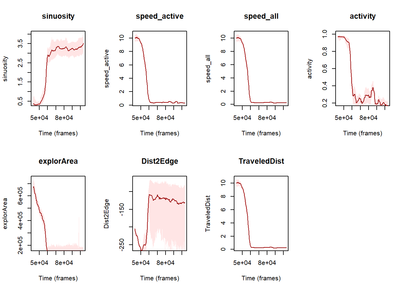
Figure 7: Evolution of the various metrics (i.e., sinuosity, speed for including active state only, speed including all activity states, activity, surface explored, distance to the edge of the arena and distance traveled by the individuals) over the experiment timeline expressed in frames.
Great! now that we have computed the studentized 95% CI, we can see that the distance to the edge is very variable (fig. 7) compared to the others metrics.
Also, as the speed metrics, the distance traveled and the surface explored exhibit very similar trends we can hence use a more synthetic view of the results by plotting the sinuosity, the activity and the speed (for all individuals) on the same plot.
# import a custom function to plot the results
source(
  "https://raw.githubusercontent.com/qpetitjean/TrichoG_Thermal_Biology/main/RScripts/Strains_plotFunc.r"
)

# plot the activity, speed and sinuosity and studentize 95% confidence interval as an envelope as well as the number of detection over the experiment.
strains_plot(
  finalDatList = trackDatL,
  smoothDf = TemporalRes_wtd,
  TempAxis = "y",
  TempCol = "Measured_Temp_Deg_C",
  TempScale = c(35,45,2),
  TimeCol = "runTimelinef",
  TimeLimit = c((25 * 60 * 25), (70 * 60 * 25)),
  nbrIndcounted = 24,
  IC = boot.ci.NoNA,
  variables = c("activity" , "speed_active", "sinuosity"),
  colvariable = c("#339999", "#6600CC", "#669933"),
  scaleVariable = list(c(0, 1, 0.2),
                       c(0, 12.5, 2.5),
                       c(0, 5, 1)),
  Lab = list("Activity (%)",
             expression("Speed (" * list(px.s ^ -1) * ")"),
             "Sinuosity"),
  cex.lab = 0.8,
  xTick = 5,
  InnerSpace = 0.51,
  YlabSpace = 1.125
)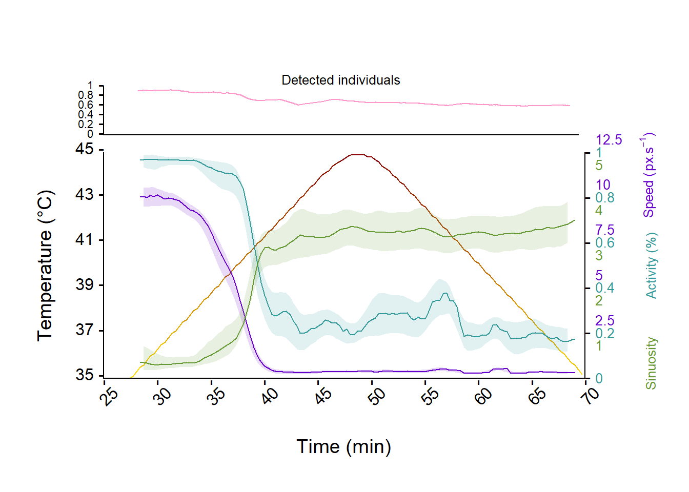
Figure 8: Evolution of the activity, sinuosity and speed of Trichogramma individuals and studentize 95% confidence interval over time and temperature ramp (from 35°C to 45°C and back to 35°C, yellow to red line). The upper panel represent the evolution of the number of detected individuals relative to the true number of individual introduced in the arena (i.e., 24) over the experiment.
Great! We now have a better look at the effect of temperature on Trichogramma’s movements (see fig. 8) and can now retrieve a temperature threshold at which movements start to decrease (about 38℃) or even stop (CTmax about 41℃).
As these computation may be relatively intensive, and hence time consuming, depending on the size of the dataset (i.e., number of individuals tracked, duration of the tracking), the amount of metrics to compute and the sampling resolution (i.e., sampling argument) specified in temporalTrend and temporalBoot, it is easily possible to run the computation in parallel (across several thread of a personal computer, tutorial in progress).
Happy coding.
References
Christian, H., (2020). fpc: Flexible Procedures for Clustering. R package version 2.2-9.
Ester, M., Kriegel H.P., Sander, J., Xu X., (1996). A Density-Based Algorithm for Discovering Clusters in Large Spatial Databases with Noise. Institute for Computer Science, University of Munich. Proceedings of 2nd International Conference on Knowledge Discovery and Data Mining (KDD-96)
Wajnberg, E., Colazza, S., (1998). Genetic variability in the area searched by a parasitic wasp: analysis from automatic video tracking of the walking path. Journal of Insect Physiology 44, 437–444. https://doi.org/10.1016/S0022-1910(98)00032-8